Ising model

Ising model is a generalized mathematical model of feromagnetism in statistical physics. In this model particles having magnetic spin are put inside vertices of graph. In general case structure of graph can vary a lot, but in the usual case selection is limited to the lattices of different dimensions. Behavior of such system is observed at different temperature in the quest to find critical temperature at which phase shift occurs. If you want to familiarize yourself more with Ising model and its various interpretations, you should read [1, 2] works, because in this text we will only consider one possible, numerical, algorithm - heat bath algorithm.

Note that this model is not only applicable towards common problems of Statistical Physics, but it also has many different interdisciplinary applications. It is true as one can put agents, generalized objects imitating seemingly human behavior, into the vertices of the graph. Thus one could analyze herding behavior in human inhabited systems (see for ex. [3, 4, 5]).

About the model

Hamiltonian of system, whose every particle can interact with other particles and with the external magnetic field, can be expressed as

\begin{equation} \mathcal{H} = - \frac{1}{2} \sum\limits_{j \neq i=1}^{N}J_{i,j} \vec S_i \vec S_j - \vec H \sum\limits_{i=1}^{N} \vec S_i , \end{equation}

here \( J_{i,j} \) - strength of interaction between two particles, \( \vec S_i \) - spin of the particle, \( \vec H \) - external magnetic field.

The above Hamiltonian is very general, thus it is simplified by making some assumptions. First it is required that spins of the particles can align themselves in parallel to the selected axis, thus \( \vec S_i \) projection on to that axis, \( s_i \), can only be equal to \( \pm 1 \). If the requirement is fulfilled, then only the projection, \( h \), of the external magnetic field, \( \vec H \), has to be considered. Also note that strength of interaction between two particles should decrease with the increasing distance between them - thus in the simplest case one can assume that particle interacts only with it's immediate neighbors. In case of 2D lattice, structure we chose, particle has 4 immediate neighbors. Thus now we can rewrite Hamiltonian as

\begin{equation} \mathcal{H_{2D}} = - J \sum\limits_{x,y} s_{x,y} \left(s_{x+1,y} + s_{x,y+1} \right) - h \sum\limits_{x,y} s_{x,y} , \end{equation}

here \( x \) and \( y \) are coordinates on 2D lattice (summations in the above Hamiltonian is made over all possible \( x \) and \( y \) values). In the original Ising model value of \( J \) is fixed and equal to 1 - modeled matter is assumed to have feromagnetic properties below critical temperature and paramagnetic above. Thus we could drop \( J \) from the above Hamiltonian, but it is kept as in the applet below we have also implemented opposite, antiferomagnetic (\( J = -1 \)), case. Though antiferomagnetic case is not very interesting as phase shift is not observed.

Temperature is introduced into the model by implementing heat bath. Each selected particle is connected to the heat bath. Afterward joint system is allowed to reach thermal equilibrium. Thus new state of the particle, direction of it's spin, is chosen based on Boltzmann distribution - probability to observe system state with energy \( E \) is proportional to \( \exp \left(- \frac{E}{k T} \right) \).

Phases and phase shift in Ising model

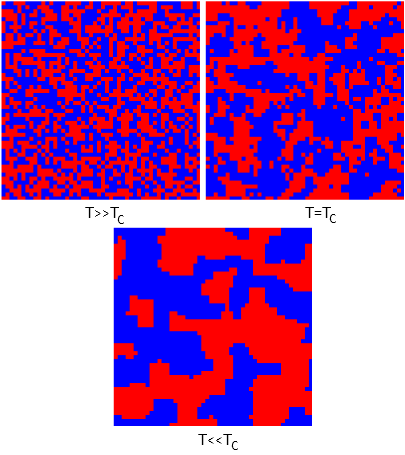
From the introduction of temperature in to the model it should be evident that model will behave differently at different temperatures - two different phases will be observed. Disorder will dominate in case of high temperature as particles will increase their own energy using thermal energy. While if temperature is low, thermal energy is also low, thus particles will not be able to increase their energy - particles will try to obtain minimal energy. In this orderly phase at first same spin domains will form and grow, while finally in the end one spin will dominate whole lattice. Most interesting behavior is observed at intermediate, critical, temperature - aforementioned two behaviors are balanced and forming orderly domains are continuously being destroyed by random spin flips. Below in Fig. 1 we present typical lattice snapshots at different temperatures.

Fig 1.Three different phases of Ising model: paramagnetic, critical, feromagnetic.

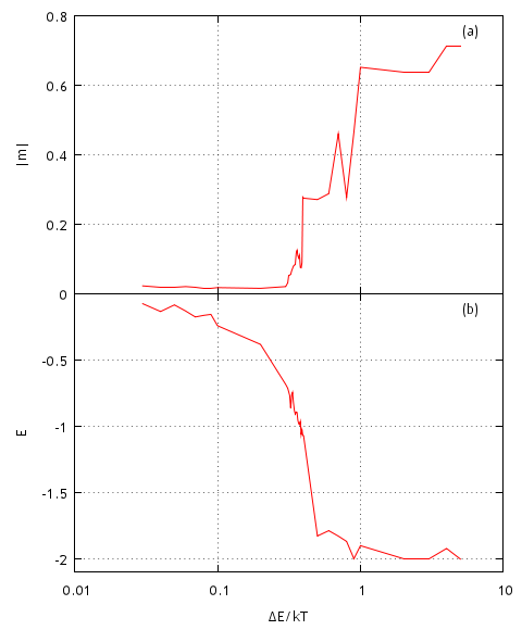
In order to numerically estimate critical temperature one must check a range of temperatures and observe how magnetization and system energy change. Below in Fig. 2 we demonstrate how the aforementioned observables change with changing model parameter \( \frac{\Delta E}{k T} \) (\( \frac{\Delta \mathcal{H}}{k T} =\frac{\Delta E}{k T} J \sum\limits_{\langle i , j \rangle} s_js_i \)), which is actually inverse temperature measured as energy in terms of spin energy. As we see from the figure phase shift occurs in the interval \( 0.3 < \left( \frac{\Delta E}{k T} \right)_c< 0.5 \).

Fig 2.System absolute magnetization (a) and energy (b) reached after \( 10^7 \) spin flips with different model parameter \( \Delta E / kT \) values.

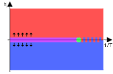
Previously we assumed that there is no external magnetic field. But how would observed model behavior change if external magnetic field is present? The answer is given in h-1/T phase diagram below (see Fig. 3) - external magnetic field aligns most of the spins in one direction (same as the direction of magnetic field).

Fig 3.h-1/T phase diagram: in the red and blue areas one spin direction dominates (s=1 (red) or s=-1 (blue)) due to the external magnetic field, paramagnetism is observed near \( h=0 \) and \( T > T_c \) (magenta area), feromagnetism is observed near \( h=0 \) and \( T < T_c \) (area colored in red-blue stripes). Critical behavior area around h=0 and \( T=T_c \) (green area).

HTML5 Applet

In the applet below we present implementation of Ising model on 50x50 2D square lattice. In the applet window you can see four figures - current spatial spin distribution graph, evolution of energy, entropy and magnetization. Single iteration corresponds to the one thousand attempts to change the spin of the random particle. After every iteration each figure is renewed. Numerical calculations are started by pressing button "Start" and can be stopped by pressing button "Stop". After stopping the calculations user can resume them or restart them from the beginning.

References

• R. J. Baxter. Exactly solved models in statistical mechanics. Academic Press Inc., Harcourt Brace Jovanovich Publishers, London, 1982. https://tpsrv.anu.edu.au/Members/baxter/book.
• J. P. Sethna. Statistical Mechanics: Entropy, Order Parameters and Complexity. Clarendon Press, Oxford, 2009. https://pages.physics.cornell.edu/sethna/StatMech/.
• S. Bornholdt. Expectation bubbles in a spin model of markets: Intermittency from frustration across scales. International Journal of Modern Physics C 12: 667-674 (2001).
• T. Kaizoji, S. Bornholdt, Y. Fujiwara. Dynamics of price and trading volume in a spin model of stock markets with heterogeneous agents. Physica A 316: 441-452 (2002).
• S. H. Yook, H. J. Kim, Y. Kim. Agent-based generalized spin model for financial markets on two-dimensional lattices. Journal of the Korean Physical Society 52: S150-S153 (2008).